Wind potential evaluation

The evaluation of the available wind potential in a potential site for a wind park’s installation is required in order to calculate in advance the expected annual electricity production from the wind park.

A first approach to the estimation of the available wind potential in a site can be performed by observing the distortion of the existing vegetation due to the wind. For example, the existence of trees bended closely to the ground by the wind can be an indubitable evidence for the existence of high wind potential. The distortion degree of the vegetation in an area represents the existing wind potential with specific indexes (see table 1) that have been defined exactly for this purpose. In figure 1 the distortion degrees are presented according to Griggs-Putnam, regarding trees of conical shape. In figure 2, the distortion degrees according to Barsch are presented, regarding trees of oval shape [1].

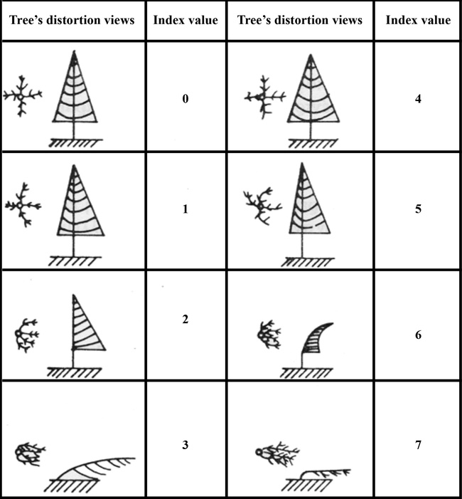
Figure 1: Distortion degree of trees according to Griggs-Putnam [1].

 

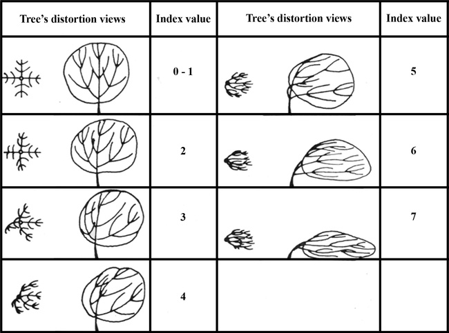
Figure 2: Distortion degree of trees according to Barsch [1].

 

 

Given the distortion degree of the trees in the examined area, the available wind potential can be estimated using table 1 [1]. As seen in this table the mean annual wind velocity in an area can be pre-estimated quite satisfactorily, with an error of ± 20-30%, on the basis of the existing vegetation distortion degree. This can be a first piece of information in the site selection procedure.

Except the above, the opinion of people living closely to the examined area can always provide important information towards the first estimation of the existing wind potential. Shepherds, farmers, fishermen with frequent presence at the vicinity of the examined site can be approached tactfully and asked generally about the existing weather conditions. Invaluable information can be gathered from local inhabitants, although special approach skills can be required.

The evaluation of the wind potential at the installation site begins with the installation of a meteorological (or wind) mast for the collection of wind potential measurements. Such measurements include the wind velocity magnitude and direction, the wind gusts etc. Wind potential measurements are received for very short time intervals (e.g. for every second) and mean measurements are recorded for certain predefined time periods, e.g. for every ten minutes. The total measurement period should be at least one year, in order to permit secure evaluation of the wind potential. The expansion of the measurement period to more than one year will certainly lead to more reliable conclusions concerning the examined wind potential. However, secure information concerning the variability of the wind versus the years can also be gathered from long-term meteorological data, recorded from satellites for specific points on earth [2, 3]. The long-term data, compared to the short-term wind potential measurements, can also provide reliable information concerning the variability of the wind potential for a time period of 2-3 decades. The wind potential evaluation based on long-term wind potential data is distinguished in the following steps:

• The long-term meteorological data, recorded from satellites, are provided for specific points on earth and for certain altitudes (approximately 100m above sea level). Two nearest points to the wind mast installation position with available long-term data are selected.
• By applying interpolation techniques, the long-term data are transferred to the wind mast installation position, taking into account the distances between the long-term data points and the wind mast position.
• The long-term data usually cover a time interval of 30 years with mean values of wind velocity magnitude and direction for every six hours. The short-term wind potential data measured by the wind mast are considered more accurate and reliable than the long-term one. The mean annual wind velocity of the short-term data is compared to the corresponding one of the long-term, for the measurements’ time period. If significant difference between these two values exhibits, then the long-term time-series is corrected analogically by multiplying its values with the ratio of the short-term over the long-term annual mean wind velocity.

The long-term meteorological data are provided by reliable institutes (e.g. N.A.S.A., N.R.E.L. etc) and can be found in specific electronic sites [2, 3]. The possession of annual wind potential measurements and long-term meteorological data can provide accurate information about the existing wind potential in the installation site, on the condition of a proper statistical correlation of the available time-series, as presented previously. In figure 3, the mean annual wind velocity variation is presented at the installation position of a meteorological mast in the Greek island of Kasos at the south east Aegean Sea, based on satellite wind potential data, calculated following the above described methodology.

 

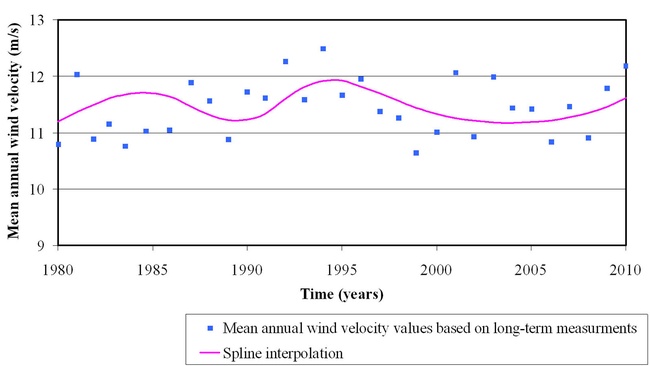
Figure 3: Mean annual wind velocity variation at the installation position of a meteorological mast, based on satellite wind potential data.

 

The fundamental feature of a wind mast is its height. The height of the wind mast is mainly implied by the expected wind potential. The height above ground where the wind boundary layer is fully developed depends on the ground roughness. Generally, the wind velocity increases with the height above ground. Consequently, the higher a meteorological mast is, the higher the measured wind velocity is expected to be. The optimum installation is a meteorological mast with height equal to the hub height of the wind turbine that will be installed. In this case, the measured wind velocity will be exactly the one that the wind turbines’ rotors will face. However, the cost of the meteorological mast increases almost linearly with its height. For example, the cost of a 10m high meteorological mast in Greece varies between 10,000 and 15,000€, depending on the specific installation position of the mast. This means that the cost for a 40m high wind mast will exceed 40,000€, while the cost of a 60m high wind mast will exceed 60,000€. In sites where the wind potential is estimated to be high beforehand, the height of the wind mast can be restricted. Namely, if the measured wind velocity in 10m height above ground exceeds a lower desirable limit set by the developer (e.g. 7.5m/s), it is sure that at the wind turbine’s hub height the wind velocity will be higher, hence it will meet the expectations of the developer. In this case the installation of a 10m high wind mast can be enough. On the other hand, if the wind velocity met in low heights is low, then a higher wind mast should be installed, in order to collect more accurate information about the available wind potential closely to the wind turbine’s hub height.

A 40m high meteorological mast is presented in figure 4 with 3 levels of measurements at 10m, 25m and 40m of height.

 

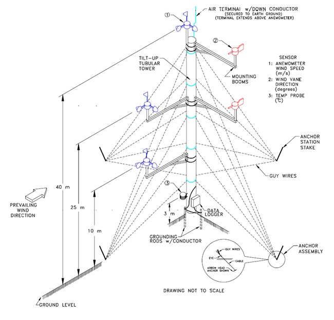
Figure 4: A 40m height meteorological mast [4].

 

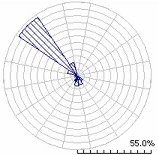
Once the measurement of the wind potential is completed, a statistical analysis of the recorded time-series is fulfilled using special software tools. Among the results of this analysis are the wind-rose diagrams or the Weibull probability density distributions of the wind velocity, for monthly time periods and for the total measurements time period. Several characteristic statistical features are also calculated, such as the wind velocity standard deviation, the mean monthly and annual values, the duration curve of the wind velocity etc. In figures 5 and 6, the annual wind-rose and Weibull probability density calculated from annual wind potential measurement time-series are presented.

 

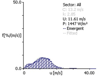Figure 5: Wind-rose based on annual wind potential measurements on a site in the island of Kasos.	Figure 6: Weibull distribution based on annual wind potential measurements on a site in the island of Kasos.

 

The gathered measurements are finally imported in specific software tools to evaluate the wind potential on the total installation site. The wind map is developed and several features are calculated, such as the Weibull C and k parameters and the wind-rose graphs in selected positions. Except the gathered time-series, other required data for the wind map development are the coordinates of the wind mast installation position, the height of the wind mast, the height above ground at which the wind flow field will be calculated (usually this is set equal to the turbine’s hub height), the ground roughness, the area boundaries of the wind flow field development etc. The wind potential is calculated in specific points of the total territory (land discrimination). The density of the calculation grid is also defined by the software’s user. By importing specific wind turbine’s model in the turbines’ installation positions, these tools can further calculate the expected annual electricity production from the wind turbines, including the energy shading losses from one wind turbine to another. More information about the calculation of the annual electricity production from a wind park is provided in a next section.

An example from a wind map developed for a specific site in the southern Crete is presented in figure 7. The position of the wind mast installation is presented at this figure, as well as a wind-rose presenting the wind main blowing direction (north). The wind measurements were gathered from 2/7/2008 to 1/7/2009. The wind potential measurements time period is one year, giving a mean annual wind velocity of 8.67m/s. The Weibull distribution parameters are calculated equal to C=9.7 m/s and k=1.77.

 

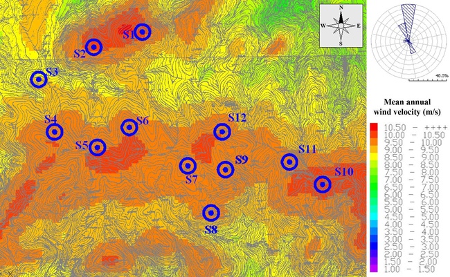
Figure 7: Wind map developed from annual wind velocity measurements for a site in the southern Crete. The abbreviation S1, S2, … stands for wind turbines’ installation sites.

 

Another wind map example is presented in figure 8, for a site in the island of Kasos, in the Dodecanese complex (south east Aegean Sea). The wind mast installation position is also depicted in this figure. The duration of the wind potential measurements is 9 months, from 14/5/2010 to 13/2/2011. The wind velocity mean value over the measurements time period is 11.61m/s. The Weibull distribution parameters are calculated equal to C=13.2m/s and k=2.85.

 

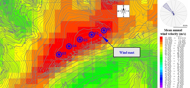
Figure 8: Wind map developed from 9-months wind velocity measurements for a site in the island of Kasos. The abbreviation S1, S2, … stands for wind turbines’ installation sites.

 

Finally a wind map developed for an offshore area in the south west of the Greek island of Rhodes is presented in figure 9, based on wind potential measurements for a six-month time period. The 10m height meteorological mast is installed in a small rocky island. The mean wind velocity is measured 9.1m/s. The Weibull distribution parameters for the annual time period are calculated equal to C=10.3m/s and k=2.2.

 

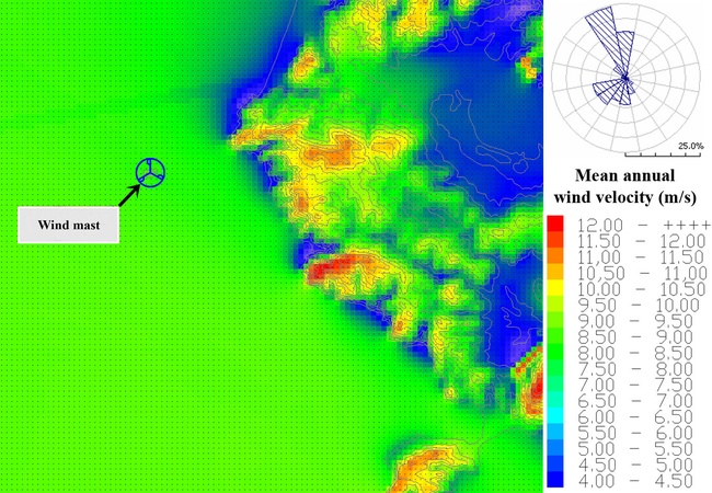
Figure 9: Wind map developed from annual wind velocity measurements for an offshore site in south west of Rhodes.

 

By comparing the wind maps presented in the above figures, the intensive effect of the land morphology on the examined wind potential is revealed. In offshore areas, the wind potential is presented uniform, without variations for different positions. The wind boundary layer is fully developed in lower altitudes and higher wind velocity values are recorded.

 

 

References

 

[1]         Bergeles G. Wind Converters., Simeon, Athens, 2005.

[2]         National Center for Environmental Prediction (NCEP). Reanalysis data provided by the NOAA/OAR/ESRL PSD, Boulder, Colorado, U.S.A. Web site at http://www.cdc.noaa.gov/

[3]         Kalnay et al., “The NCEP/NCAR 40-year reanalysis project”, Bull. Amer. Meteor. Soc., 77, 437-470, 1996.

[4]         AWS Scinetific Inc. National Renewable Energy Laboratory. Wind resource assessment handbook. Fundamentals for conducting a succesfull monitoring program. April 1997.