Wind park's annual electricity production

The calculation of the annual electricity production from the wind park is performed after the wind potential evaluation and the wind map development on the installation site and the final micro-siting of the wind turbines. The calculation of the annual electricity production from the wind park will enable the estimation of the annual electricity vending to the utility and the expected annual revenues from the investment.

The annual electricity production from the wind park is calculated by specialised software tools. The development of the wind map provides information about the available wind potential at the specific installation positions of the wind turbines. This information may be provided with the Weibull distribution parameters C and k or with annual wind velocities time-series at each installation position etc. Giving this information, the annual electricity production from each wind turbine is calculated by introducing the power curve of the selected wind turbine model.

In figure 1 a typical power curve of a 850kW nominal power wind turbine is presented, while in figure 2 a wind velocity Weibull probability density annual distribution is presented.

 

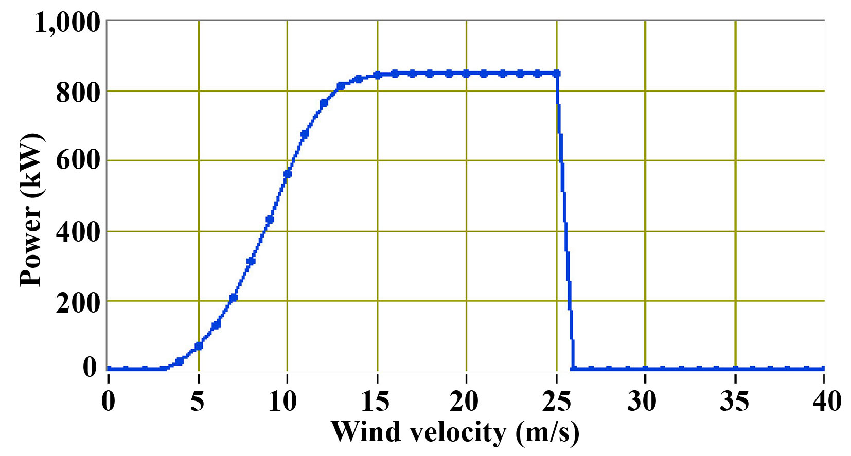
Figure 1: The power curve of a 850kW nominal power wind turbine.

 

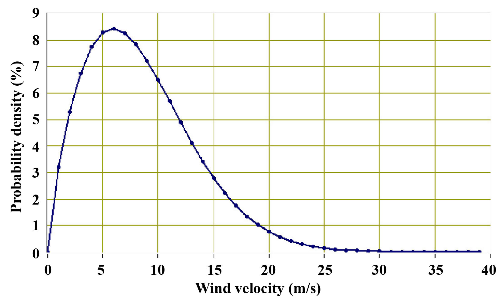
Figure 2: A wind velocity Weibull probability density distribution.

 

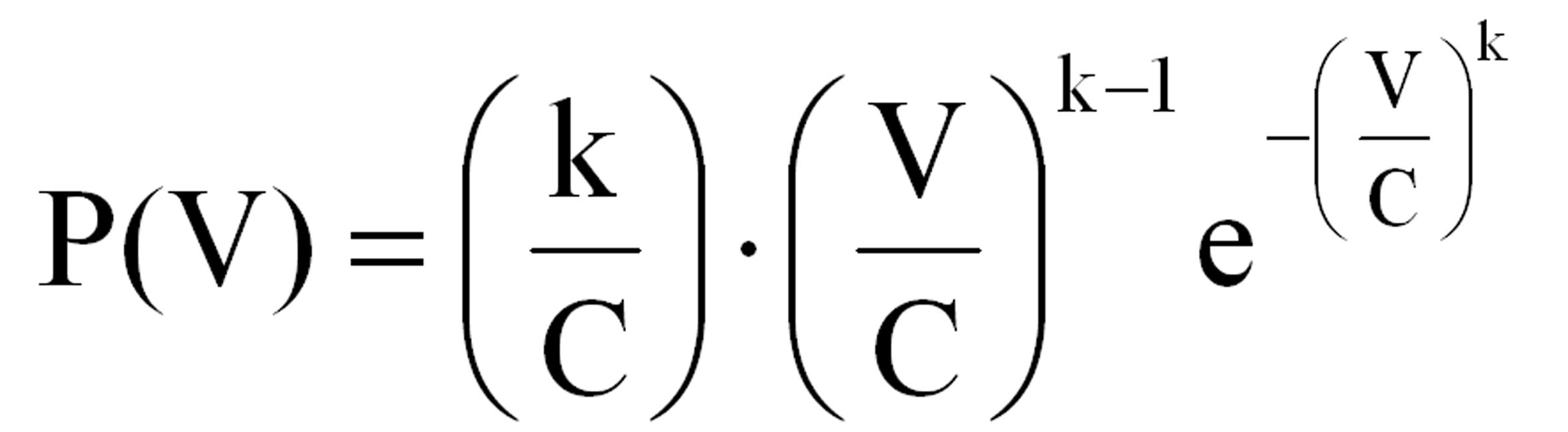
The Weibull probability density distribution is given by the following relationship:

 

(1)

 

The Weibull parameters C and k depend respectively on the wind velocity averaged value and the dispersion of the wind velocity values. They are called as Ονομάζονται αντίστοιχα παράμετρος μεγέθους και παράμετρος μορφής. In relationship 1 V is the wind velocity independent variable. Different wind velocity time series give different probability density distribution, which are approached with the Weibull empirical relationship, versus the Weibull parameters C and k.

In table 1 the calculation of the annual electricity production from a wind turbine, based on the wind turbine power curve and the wind velocity Weibull probability density distribution is presented. The calculation procedure presented in table 1 is simple. For each wind velocity interval there is one corresponding Weibull probability value and one wind power output from the wind turbine’s power curve. The Weibull probability density value corresponds to a total number of hours per year that the wind blows taking values inside the specific wind velocity range. The wind turbine’s power curve implies a specific power output during these hours.  The product of the total hours per year with the power output from the wind turbine gives the total annual electricity production for each wind velocity interval. The sum of the electricity production from all the wind velocity intervals estimates the expected total annual electricity production from the wind turbine.

 

 

 

 

In the example presented in table 1, the annual electricity production from the 850kW wind turbine installed in a site with the specific wind speed Weibull density distribution is calculated equal to 3,183,184kWh.

The annual capacity factor of the wind turbine is defined as the ratio of the turbine’s annual electricity production over the maximum theoretical one. The annual maximum theoretical production is based on the condition that the power output of the wind turbine remains constant and equal to its nominal power for the whole year. In this case, the expected electricity production is calculated equal to 850kW x 8,760h = 7,446,000kWh. The annual capacity factor is then calculated equal to CF= 3,183,184kWh / 7,446,000kWh = 42.75%.

From the above presented analysis it is obvious that the capacity factor depends on:

·         the selected wind turbine model

·         the available wind potential, consequently the selected installation site

·         the time period over which it is calculated.

Above all, the capacity factor depends on the available wind potential and comprises a characteristic index of the wind potential quality of a site. Different sites exhibit different capacity factors. The capacity factor of 42.75% calculated previously is considered high. Such values are met in sites with high wind potential, such the ones met in some of the Greek islands or in the Scottish coast. In central Europe common values for capacity factor are between 25 and 30%.

The first results regarding the annual electricity calculation are provided for each wind turbine in a form given in the example of table 2. The wind potential evaluation and the annual electricity production are the first set of results. The results in table 2 refer to a 21MW wind park installed in the southern Crete. As shown in this table, the annual energy production, calculated by the relevant software, has taken into account the wind turbines shading losses. In order to conclude to the final electricity vended to the utility, the following further losses, except the wind turbines shading losses, must be calculated:

·         wind turbines’ hysteresis losses

·         electricity transportation losses

·         losses due to wind turbines’ technical unavailability

·         losses due to wind power rejection from the utility (mainly in non-interconnected systems).

 

 

 Each wind turbine cuts out its operation over a wind velocity value, set by the manufacturer usually at 25m/s, in order to protect itself. If the wind velocity exceeds this upper operation limit, the wind turbine stops operation immediately. The wind turbine will start operating again after a certain time interval, configured by the manufacturers, during which the wind velocity must remain under the upper operation limit. During this time interval, the available wind energy is not exploited and the electricity that could be produced corresponds to the energy hysteresis losses. The hysteresis losses depend on the variation of the wind velocity in the turbines’ installation positions. Hence the calculation of the hysteresis losses is based on the available wind potential information (wind velocity time-series or Weibull probability density distribution) for every turbine’s installation position.

The electricity transportation losses are caused by the network ohmic, inductive and capacitive resistance. These resistances depend on the existing network’s distance from the wind park to the connection point, the connection line voltage, the conductors’ cross-section etc and can be calculated accurately. Usually the electricity transportation losses vary between 3-5%, for the most usual cases, although in wind parks with very long connection networks (higher than 100km) these losses can exceed 5%.

The wind turbines are not always technically available, due to either unpredicted operational damages or scheduled maintenance. The technical availability of a wind park is usually guaranteed by the turbines’ manufacturer, within the purchase and maintenance contract that is signed between the manufacturer and the wind park’s owner. The technical availability of a wind park is expressed as the operational time percentage during a year over the total annual time period. This feature can exceed 98% in case of easily accessed wind parks. In case of offshore wind park this feature usually reduces below 95%.

Finally, in case of wind parks installed in isolated power systems, there is always an upper limit of wind power penetration in the electricity production system. This upper limit is set in order to ensure the isolated system’s dynamic security and stability. The maximum instant wind power penetration over the power demand percentage is usually set equal to 30%, following the results of relevant simulations [1-3]. Except the upper limit of wind power penetration, wind power rejection is also caused from the restrictions introduced in the system’s operation by the on-duty thermal generators technical minima. Depending on the power demand size and on the total wind power installed in an isolated system, wind power rejection due to violation of the upper wind power penetration limit or to technical minima restrictions can occur. The wind power rejection from the utility network is not easily calculated. It requires the accurate simulation of the system’s annual operation, based on annual time-series of power demand and wind power production mean hourly values.

In figure 3, an analysis of the calculation of the final electricity production from the 21MW wind park installed in the southern Crete is provided. The calculation starts from the energy production after wind turbines’ shading losses and following all the energy losses calculations presented above, concludes to the final electricity production that is purchased by the utility. The wind turbines’ availability is set equal to 95%, following the relevant warranty of the manufacturers. The electricity transportation losses, through a 20kV underground 20km long cable are estimated approximately 3%. The hysteresis losses are calculated accurately on the basis of wind potential measurements gathered by a 10m meteorological mast installed at the specific site. The wind power rejection losses are also calculated accurately with the simulation of the system’s annual operation, based on annual time series of the power demand and the wind power production. Finally, the turbines’ shading losses are calculated directly by the specialised commercial software tool through which the wind potential evaluation and the wind map analysis of the installation site are also accomplished.

 

 

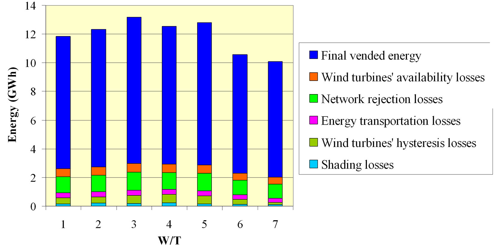
Figure 3: Energy production analysis from a 21MW nominal power wind park.

 

The energy production calculation can be integrated with an uncertainty analysis regarding the probability the annual wind park’s energy production to exceed several values. The uncertainty analysis is accomplished on the basis of the short-term wind potential data measured by the installed meteorological mast and long-term wind potential data gathered by satellites from specific points on earth and heights above grounds. As mentioned above, the long-term wind potential data are transferred to the installation position of the meteorological mast using simple linear interpolation methods

The uncertainty analysis takes into account several parameters that increase the uncertainty of the energy production calculation. Such parameters are the accuracy of the anemometers on the meteorological mast, the accuracy of the wind map development, the accuracy of the several losses calculation, the accuracy of the wind turbine’s power curve etc. The final result of the uncertainty analysis is the uncertainty curve presenting the probability the electricity annual production to exceed a specific value. Such a curve is provided in figure 4, regarding a wind park of 4.5MW nominal power in the island of Kasos (Dodecanese complex, southeast Aegean Sea).

 

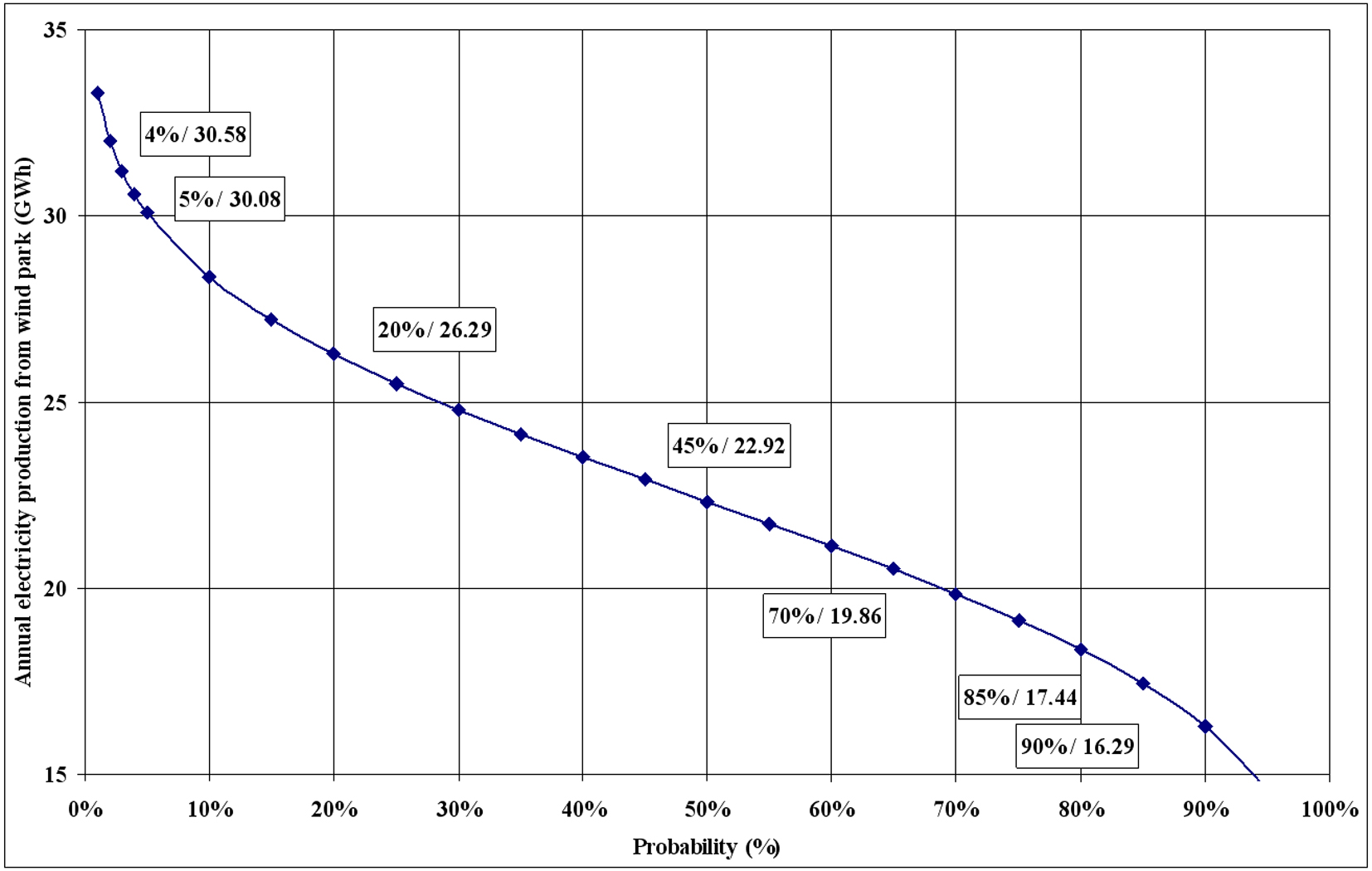
Figure 4: Probability variation for the annual net electricity production from the wind park, based on long-term wind potential data.

 

The calculation of the annual energy production from a wind park, based on short-term wind potential annual measurements, accompanied with the uncertainty analysis based on long-term data, provides secure information about the expected annual energy production and the investment’s financial efficiency.

 

 

References

 

[1]          Dialynas E. N., Hatziargyriou N. D., Koskolos N., Karapidakis E. Effect of high wind power penetration on the reliability and security of isolated power systems, paper 38-302, 37th session, CIGRÉ, 30th August – 5th September 1998.

[2]          Hatziargyriou N., Papadopoulos M. Consequences of high wind power penetration in large autonomous power systems, CIGRÉ Symposium, Neptum, Romania, 18-19 September 1998.

[3]          Sørensen Poul, Unnikrishnan A.K., Mathew Sajan A. Wind farms connected to weak grids in India, Wind Energy, 4, 137-149, 2001.